Symbolic Circuit Analysis

Symbolic Circuit Analysis using matlab  (http://ricknewby.blogspot.tw/)

Lately I’ve been working on ways to integrate Matlab and Spice simulation. While I was browsing Matlab file exchange I ran into some rather fascinating software. It’s called SCAM, which stands for Symbolic Circuit Analysis in Matlab. This a Matlab script that provides symbolic solutions to circuits; it works with resistors, capacitors, inductors and opamps.

Despite the unfortunate name (seriously, who names their product SCAM?), I found the script to be very useful. The way it works is that you first define a circuit using a netlist, in the style of Spice. Then the script solves the circuit and produces the results in symbolic form. The creators of this software also offer a tutorial on how to use Symbolic Circuit Analysis in Matlab.

What I really like about this is that you can get actual equations from your simulation, not just a graph or numerical data. To show you an example of what SCAM is capable of let's analyze the sample circuit below. Let's say we want to find the transfer function, where the output voltage is the voltage at node 5.

Finding Vout/Vin

Step 1: Create a Netlist

The first thing that we need to do is create a netlist. To create a netlist you can just use a basic text editor, like notepad or the far superior notepad++, and you have to save it with the *.cir extension. The syntax is very similar to Spice:

So, for this example we end up with the following netlist:

Notice how some components don't have numeric values? This is one of the nicer features of of SCAM, we can do an analysis and simulation without having all of the component values.  

Step 2: Run the Analysis

To run the simulation you need to enter the following commands:

Before you can call the main script, you have to set the variable fname to the path of your netlist. In this case, the netlist is in the same folder as the script, so the path is just the file name. The output from these commands was:

As you can see, we now have the voltages for each node. Let's calculate our transfer function, recalling the output voltage was node 5:

Here the transfer function is stored into the variable H, and the collect function is just grouping terms together by power.

Now let's take a look at the results, first the symbolic equation. To print the transfer function we can use the pretty function, which displays the equation in an easy to read format:

This gives the following output:

To see the numeric solution, we can use the eval function to replace the symbols with their actual values:

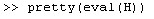
This time the result was:

And there you have it, in a just a few lines of code we were able to generate an actual equation for our transfer function. Pretty cool!

Downloads

• Script and sample netlists 

Symbolic Circuit Analysis using mathmatica

Symbolic Circuit Analysis with Analog Insydes

http://library.wolfram.com/examples/AnalogInsydesSymbolic/

To execute this notebook you need the add-on package Analog Insydes by ITWM (see copyright message at end of document).

Introduction

Symbolic circuit analysis is known to yield extremely large 
expressions even for small circuits. To cope with expression 
complexity, Analog Insydes provides special functionality for calculating simplified symbolic formulas which are small and easy to understand. Approximated symbolic expressions are computed by dropping numerically insignificant terms from circuit equations or transfer functions. Consider, for example, the common-emitter small-signal amplifier shown below. We will compute a simplified symbolic transfer function that contains only those terms which have dominant influence on the passband voltage gain. 

 
Common-Emitter Amplifier 

Netlist and Models

First, we write a netlist of the circuit, specifying both symbolic and numerical values for the circuit elements. The numerical values are needed later as reference values for deciding which terms are important and which ones can be neglected.

In[1]:= << tt>
In[2]:= ceamp =  
Circuit[  
        Netlist[  
        {V1,{1, 0}, 1}, (* Unit signal at input *)  
        {VCC, {6, 0}, Type -> VoltageSource, Value -> 0},  
        {C1,{1, 2}, Symbolic -> C1, Value -> 1.*^-7},  
        {R1,{2, 6}, Symbolic -> R1, Value -> 1.*^5},  
        {R2,{2, 0}, Symbolic -> R2, Value -> 4.7*^4},  
        {RC, {6, 3}, Symbolic -> RC, Value -> 2.2*^3},  
        {RE, {4, 0}, Symbolic -> RE, Value -> 1.*^3},  
        {C2,{3, 5}, Symbolic -> C2, Value -> 1.*^-6},  
        {RL, {5, 0}, Symbolic -> RL, Value -> 4.7*^4},  
        {Q1,{2 -> B, 3 -> C, 4 -> E},  
            Model -> NPNTransistor, Selector -> ACdynamic,  
            RBN -> 1.*^3, CMN -> 1.*^-11, betaN -> 200.,  
            RON -> 1.*^4}],  
        Model[  
            Name -> NPNTransistor,  
            Selector -> ACdynamic,  
            Ports -> {B, C, E},  
            Parameters -> {RB, CM, beta, RO, RBN, CMN,  
            betaN, RON},  
       Definition ->  
          Netlist[  
          {RB, {X, E}, Symbolic -> RB, Value -> RBN},  
          {CM, {B, C}, Symbolic -> CM, Value -> CMN},  
          {CC, {B, X, C, E}, Symbolic -> beta, Value -> betaN},  
          {RO, {C, E}, Symbolic -> RO, Value -> RON} ] ] ]  
                                       //ExpandSubcircuits;  



Symbolic Calculations
If we compute the exact symbolic transfer function, we obtain an expression with more than 100 terms. This expression yields absolutely no insight into circuit behavior.  

In[3]:=ceampmna =
CircuitEquations[ceamp, SymbolicValues -> True];  
MatrixForm/@ceampmna  
Out[3]=  

In[4]:=  

vout=Together[V$5 /. First[SolveCircuitEquations[ceampmna, V$5]]]
Out [4]=  

In[5]:= Length[Denominator[vout]]+Length[Numerator[vout]]
Out[5]= 105

Simplification before Generation
To find a simple expression for the passband voltage gain, we use Analog Insydes' symbolic approximation functionality to approximate the system of circuit equations with respect to a frequency point in the passband (here ) and the given numerical element values. We allow for a maximum approximation error of 10% in that point.  


In[6]:= designpoint=MakeDesignPoint[ceamp]

In[7]:= dp2={Join[designpoint,  
              {s -> N[2 pi]*I * 10^3, MaxError -> 0.1}]}  



In[8]:= approxceamp=ApproximateMatrixEquation[ceampmna, dp2, V$5];  
MatrixForm/@approxceamp  
Out[8]=  

In[9]:= voutsimp =
V$5/.First[SolveCircuitEquations[approxceamp, V$5]]//Simplify

Approximation yields a very simple expression for the voltage gain: . To see if this expression is valid, we compare it graphically with the exact expression.  

In[10]:= voutexactn[s_]=vout/.designpoint;
In[11]:= voutsimpn[s_]=voutsimp /.designpoint;
In[12]:= BodePlot[
    {voutexactn[N[2 pi] I f], voutsimpn[N[2 pi] I f]},
    {f, 1, 10^9},
    MagnitudeDisplay -> Linear,
    PlotRange -> {{0, 2.5}, Automatic},
    PlotStyle -> {{RGBColor[1, 0, 0]},{RGBColor[0, 1, 0],
Dashing[{0.03, 0.03}]}}]
  


Out[12]= -GraphicsArray-
The above Bode plot shows that the approximated expression matches the original transfer function well within 10% tolerance at . Indeed,  is the well known gain formula for this type of amplifier. With Analog Insydes you can extract this and other design formulas automatically.  

Simplification after Generation
While equation-based approximation (SBG) can reduce the complexity of a symbolic expression greatly, the result may still contain some insignificant terms. So it is generally a good idea to apply solution-based simplification (SAG) to such a transfer function as well in order to remove the remaining irrelevant contributions. The following example demonstrates the combination of SBG and SAG.  


First, we use matrix approximation to compute a reduced-order transfer function of the amplifier that is valid for the passband and also for low frequencies. Therefore, we add a second reference point at  to the list of design points.  

In[13]:= dp3={Join[designpoint, {s -> N[2 pi]*I * 10^3,  
MaxError -> 0.1}],  
Join[designpoint, {s -> N[2 pi]*I * 10^2, MaxError -> 0.1}]};  

In[14]:= approxceamp2=  
ApproximateMatrixEquation[ceampmna, dp3, V$5];  

In[15]:= voutsimp2 =  
V$5/.First[SolveCircuitEquations[approxceamp2, V$5]]//Together  


Now, we can apply solution based approximation to compute a simplified transfer function that is more compact than the SAG-only solution and valid over a larger frequency range than the first SBG result.

In[16]:= voutsimp3=
ApproximateTransferFunction[voutsimp2,s,designpoint,0.1]//Simplify

The above result is very useful because it allows for reading off approximate symbolic expressions for the poles. To calculate these explicitly, we must solve the denominator of the transfer function for s:  


In[17]:= Solve[Denominator[voutsimp3]==0,s]

Finally, we plot this simplified transfer function together with the original function to visualize the effects of our low-and-mid-frequency approximation. The Bode plot shows that the approximation is valid from zero frequency to the  
upper end of the passband at about . High-frequency effects are not described because we did not specify a design point in the frequency region beyond the passband.  


In[18]:= voutsimp3n[s_]=voutsimp3 /.designpoint;
In[19]:= BodePlot[  
    {voutexactn[N[2 pi] I f],voutsimp3n[N[2 pi] I f]},  
    {f, 1, 10^9},  
    MagnitudeDisplay -> Linear,  
    PlotRange -> {{0, 2.5}, Automatic},  
    PlotStyle -> {{RGBColor[1, 0, 0]},{RGBColor[0, 1, 0],  
                                   Dashing[{0.03, 0.03}]}}]  
  

Out[19]= -GraphicsArray-

Copyright © 1998 by ITWM e.V.
Written by Thomas Halfmann  

Analog Insydes  
ITWM - Institut für Techno- und Wirtschaftsmathematik e.V.  
Erwin-Schrödinger-Str.  
D-67663 Kaiserslautern, Germany  

Analog Insydes is a trademark of ITWM.  
Mathematica is a registered trademark of Wolfram Research, Inc. All other product names are trademarks of their respective owners.  

Copying and redistribution of this notebook is welcomed and encouraged, provided that the entire contents of the document, in particular the above copyright notice, are left unchanged and that the file is redistributed free of charge. 

http://www.personal.rdg.ac.uk/~stsgrimb/analysis.htm

Symbolic Analysis of Electronic Circuits

As the name implies, symbolic circuit analysis generates network functions (voltage transfer function, input impedance, transadmittance) in terms of circuit symbols. Consider the Sallen-Key low-pass filter:



The symbolic form of the voltage transfer function for this circuit is:

Numerator:
+ s^ 0
Number of terms = 1

Denominator:
+ s^ 0
+ R2 * C2 * s^ 1
+ R1 * C2 * s^ 1
+ R1 * R2 * C1 * C2 * s^ 2
Number of terms = 4

Substituting the component values R1=10.0kohm, R2=10.0kohm, C1=288.8nF and C2=0.9369nF into the symbolic form gives the numerical form of the voltage transfer function:

Numerator:
a 0 = 1.0000000E+0
a 1 = 0.0000000E+0
a 2 = 0.0000000E+0

Denominator:
b 0 = 1.0000000E+0
b 1 = 1.8738000E-5
b 2 = 2.7057672E-8

Finally, substituting the frequency into the numerical form of the transfer function gives the voltage gain and phase:

 Frequency     Gain    Phase
1.000000E+2    0.09    -0.68
3.162278E+2    0.97    -2.39
1.000000E+3   17.33  -120.08
3.162278E+3  -19.73  -177.80
1.000000E+4  -40.49  -179.36

The use of symbolic network functions enormously reduces the amount of computation required to calculate, for example, the voltage gain at a number of frequencies. Instead of inverting the complex Y-matrix for each frequency it is simply necessary to substitute the frequency into the numerical form of the voltage transfer function.

Symbolic circuit analysis methods should generate the symbolic terms of the network functions efficiently and without duplication (no cancelling terms). There are two established methods for symbolic circuit analysis: the signal flow graph method and the two-graph method. I use the latter.

The two-graph method is based on the voltage and current graphs of the circuit (which correspond to the voltage and current incidence matrices of the circuit). After coalescing appropriate nodes in the two graphs, the symbolic terms are found by enumerating the common spanning trees of the two graphs (Electronic Letters).

The two-tree method for symbolic circuit analysis can be applied to passive circuits, circuits containing voltage-controlled current-sources, infinite-gain operational amplifiers (Electronic Letters) and current conveyors (Electronic Letters).

A symbolic circuit analysis program TOPCAP which uses a Spice-like netlist is available for download.

Symbolic Circuit Analysis in MatLab (SCAM) 

http://www.swarthmore.edu/NatSci/echeeve1/Ref/mna/MNA6.html